DEVELOPER’s BLOG
技術ブログ
pythonでEfficientNet + Multi Output を使って年齢予測の実装

ディープラーニングを使って、人の顔の画像を入力すると 年齢・性別・人種 を判別するモデルを作ります。
身近な機械学習では1つのデータ(画像)に対して1つの予測を出力するタスクが一般的ですが、今回は1つのデータ(画像)で複数の予測(年齢・性別・人種)を予測します。
実装方法
学習用データ
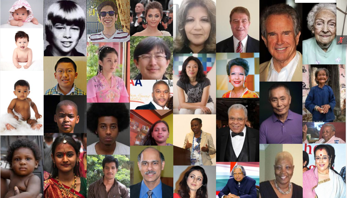
まず、学習用に大量の顔画像が必要になりますが、ありがたいことに既に公開されているデータセットがあります。 UTKFace というもので、20万枚の顔画像が含まれています。また、年齢(0-116歳)、人種(白人、黒人、 アジア系、インド系、その他)、性別はもちろんですが、表情や画像の明るさ・解像度も多種多様なものがそろっています。
モデル
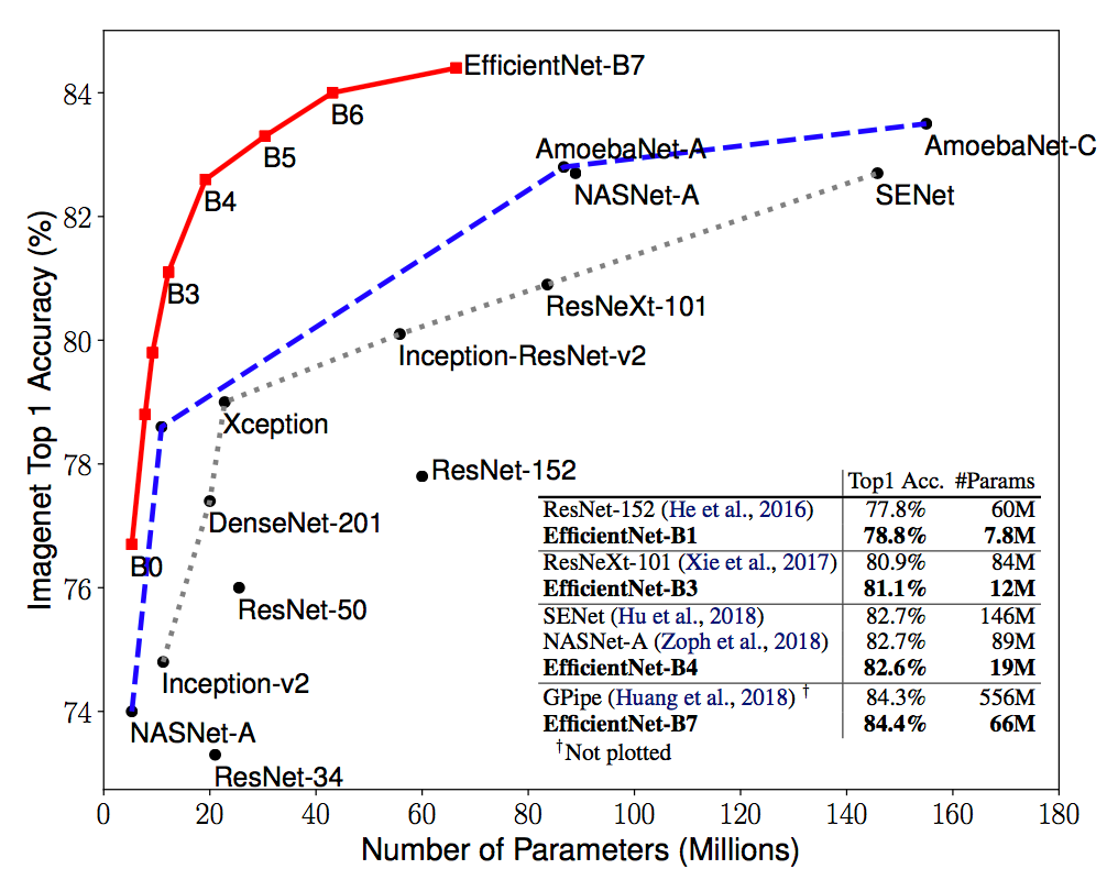
次に予測モデルについてですが、Efficient Net という2019/5月に Googleが発表したモデルを使います。このモデルは従来よりかなり少ないパラメータ数ながら、高い精度を誇る優れたモデルです。Kaggleのようなコンテストでも既に多用されていて、上位の人たちの多くが使っています。(参考:このコンテストでは上位陣の多くがEfficient Netを取り入れていました 詳しくは元論文や、その解説記事を参考にしてください。
加えて、今回のタスクは1つの入力(顔画像)から3つの出力(年齢・性別・人種)を返す、いわゆる複数出力型(Multi Output)にする必要があることにも注意します。
実装例
プログラミング環境 いくらEfficient Netの計算コストが小さいとはいっても、学習データの数も多く普通のCPUでは時間がかかりすぎてしまいます。専用GPU付PCがあればそれで良いのですが、私はないのでGoogle Colaboratoryのような外部のGPUを使う必要があります。実はKaggleにもGPU提供の機能があり、しかもKaggleの場合、あらかじめデータセットがNotebookに読み込まれている場合があります。つまり、配布元のサイトからデータをダウンロードしてくる必要がありません。今回使うUTKFaceも既に用意されているので、ありがたくこれを使っていきます。
まず、ここに行き、右にあるNew Notebookをクリックします。

今回はPythonで実装するので、そのまま createを選択します。しばらくするとデータが読み込まれた状態のNotebookが使えるようになります。これで環境構築は完了です。
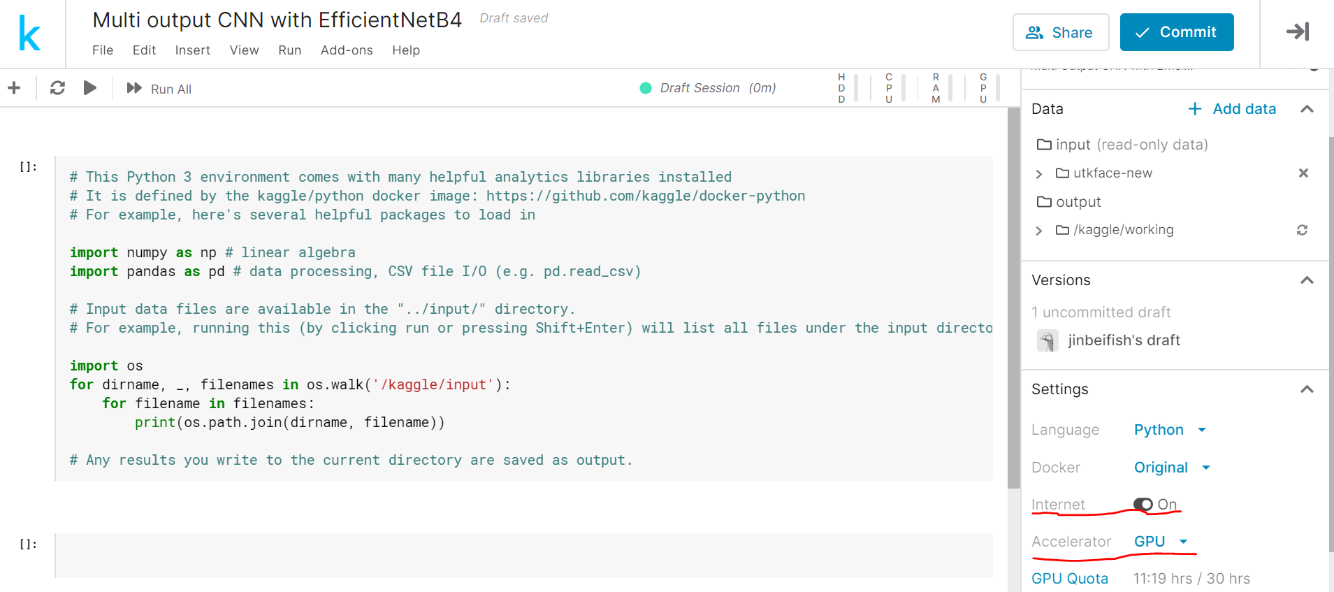
この時、図のように、【Settings】の項目のうち、 Internet を On に、Accelerator を GPU に設定 しておきましょう。
コード全文
それではいよいよ実装していきます。ここでは、最初にコード全文を載せ、後で詳細に解説していきたいと思います。
# This Python 3 environment comes with many helpful analytics libraries installed
# It is defined by the kaggle/python docker image: https://github.com/kaggle/docker-python
# For example, here's several helpful packages to load in

import numpy as np # linear algebra
import pandas as pd # data processing, CSV file I/O (e.g. pd.read_csv)

# Input data files are available in the "../input/" directory.
# For example, running this (by clicking run or pressing Shift+Enter) will list all files under the input directory

import os
for dirname, _, filenames in os.walk('/kaggle/input'):
    for filename in filenames:
        print(os.path.join(dirname, filename))

# Any results you write to the current directory are saved as output.


###### EfficientNetをインストール
! pip install -U efficientnet


###### 必要なライブラリを読み込む
import glob
import matplotlib.pyplot as plt
import seaborn as sns
from PIL import Image

from efficientnet.keras import EfficientNetB4  # Bの後の数字を変えれば別のスケールのモデルを使える
from sklearn.model_selection import train_test_split
from keras.utils import to_categorical

from keras.layers import Input, Dense
from keras.models import Model
from keras.callbacks import ModelCheckpoint


###### 定数を定義
DATA_DIR = '../input/utkface-new/UTKFace'
IM_WIDTH = IM_HEIGHT = 198
TRAIN_TEST_SPLIT = 0.01  # 全体の8割を訓練データ、残り2割をテストデータにする
TRAIN_VALID_SPLIT = 0.7  # 訓練データのうち3割はバリデーションデータとして使う
ID_GENDER_MAP = {0: 'male', 1: 'female'}  # IDから性別へ変換するマップ
GENDER_ID_MAP = dict((g, i) for i, g in ID_GENDER_MAP.items())  # IDと性別の逆引き辞書
ID_RACE_MAP = {0: 'white', 1: 'black', 2: 'asian', 3: 'indian', 4: 'others'}  # IDから人種へ変換するマップ
RACE_ID_MAP = dict((r, i) for i, r in ID_RACE_MAP.items())  # IDと人種の逆引き辞書


###### ファイル名から正解ラベルを取り出す関数
def parse_filepath(filepath):
    # 年齢(int)、性別(str)、人種(str) を返す
    try:
        path, filename = os.path.split(filepath)  # 相対パスからファイル名を取り出す
        filename, ext = os.path.splitext(filename)  # 拡張子を除く
        age, gender, race, _ = filename.split("_")  # _は無名変数
        return int(age), ID_GENDER_MAP[int(gender)], ID_RACE_MAP[int(race)]

    except Exception as e:  # いくつか欠損値があるので例外処理をしておく
        print(filepath)
        return None, None, None


###### 年齢、性別、人種、ファイル名からなるDataFrameを作成
files = glob.glob(os.path.join(DATA_DIR, "*.jpg"))  # 全ての画像ファイル名をfilesという変数にまとめる
attributes = list(map(parse_filepath, files))  # 上で作成した関数にファイル名を一つずつ入力

df = pd.DataFrame(attributes)
df['file'] = files
df.columns = ['age', 'gender', 'race', 'file']
df = df.dropna()  # 欠損値は3つ
df['gender_id'] = df['gender'].map(lambda gender: GENDER_ID_MAP[gender])
df['race_id'] = df['race'].map(lambda race: RACE_ID_MAP[race])

# 10歳以下、65歳以上の人の画像は比較的少ないので使わないことにする
df = df[(df['age'] > 10) & (df['age'] < 65)]
# その中での最高年齢
max_age = df['age'].max()

###### train, test, validationデータの分割
p = np.random.permutation(len(df))  # 並び替え
train_up_to = int(len(df) * TRAIN_TEST_SPLIT)
train_idx = p[:train_up_to]
test_idx = p[train_up_to:]

# split train_idx further into training and validation set
train_up_to = int(train_up_to * TRAIN_VALID_SPLIT)
train_idx, valid_idx = train_idx[:train_up_to], train_idx[train_up_to:]


###### データの前処理を行う関数
def get_data_generator(df, indices, for_training, batch_size=32):
    # 処理した画像、年齢、人種、性別をbatch_sizeずつ返す

    images, ages, races, genders = [], [], [], []
    while True:
        for i in indices:
            r = df.iloc[i]
            file, age, race, gender = r['file'], r['age'], r['race_id'], r['gender_id']
            im = Image.open(file)
            im = im.resize((IM_WIDTH, IM_HEIGHT))
            im = np.array(im) / 255.0  # 規格化
            images.append(im)
            ages.append(age / max_age)  # 最大年齢で規格化
            races.append(to_categorical(race, len(RACE_ID_MAP)))  # kerasの仕様に合わせ、one-hot表現に
            genders.append(to_categorical(gender, 2))  # kerasの仕様に合わせ、one-hot表現に
            if len(images) >= batch_size:  # メモリを考慮して少しずつ結果を返す
                yield np.array(images), [np.array(ages), np.array(races), np.array(genders)]
                images, ages, races, genders = [], [], [], []
        if not for_training:
            break


###### モデルの作成
input_layer = Input(shape=(IM_HEIGHT, IM_WIDTH, 3))  # 最初の層

efficient_net = EfficientNetB4(
    weights='noisy-student',  # imagenetでもよい
    include_top=False,  # 全結合層は自分で作成するので要らない
    input_tensor = input_layer,  # 入力
    pooling='max')

for layer in efficient_net.layers:  # 転移学習はしない
    layer.trainable = True

# 複数出力にする必要があるので、efficientnetの最終層から全結合層3つを枝分かれさせる
bottleneck=efficient_net.output

# 年齢の予測
_ = Dense(units=128, activation='relu')(bottleneck)
age_output = Dense(units=1, activation='sigmoid', name='age_output')(_)

# 人種の予測
_ = Dense(units=128, activation='relu')(bottleneck)
race_output = Dense(units=len(RACE_ID_MAP), activation='softmax', name='race_output')(_)

# 性別の予測
_ = Dense(units=128, activation='relu')(bottleneck)
gender_output = Dense(units=len(GENDER_ID_MAP), activation='softmax', name='gender_output')(_)

# efficientnetと全結合層を結合する
model = Model(inputs=input_layer, outputs=[age_output, race_output, gender_output])

# 最適化手法・損失関数・評価関数を定義してコンパイル
model.compile(optimizer='rmsprop',
              loss={'age_output': 'mse', 'race_output': 'categorical_crossentropy', 'gender_output': 'categorical_crossentropy'},
              loss_weights={'age_output': 2., 'race_output': 1.5, 'gender_output': 1.},
              metrics={'age_output': 'mae', 'race_output': 'accuracy', 'gender_output': 'accuracy'})

# バッチサイズを定義
batch_size = 32
valid_batch_size = 32

train_gen = get_data_generator(df, train_idx, for_training=True, batch_size=batch_size)
valid_gen = get_data_generator(df, valid_idx, for_training=True, batch_size=valid_batch_size)

# 検証誤差が最も低い状態のモデルを保存しておく
callbacks = [
    ModelCheckpoint('./model_checkpoint', monitor='val_loss', verbose=1, save_best_only=True, mode='min')
]

history = model.fit_generator(train_gen,
                    steps_per_epoch=len(train_idx)//batch_size,
                    epochs=10,
                    callbacks=callbacks,
                    validation_data=valid_gen,
                    validation_steps=len(valid_idx)//valid_batch_size)


###### 損失関数、評価関数の値をプロットする関数
def  plot_train_history(history):
    fig, axes = plt.subplots(1, 4, figsize=(20, 5))
    axes[0].plot(history.history['race_output_accuracy'], label='Race Train accuracy')
    axes[0].plot(history.history['val_race_output_accuracy'], label='Race Val accuracy')
    axes[0].set_xlabel('Epochs')
    axes[0].legend()

    axes[1].plot(history.history['gender_output_accuracy'], label='Gender Train accuracy')
    axes[1].plot(history.history['val_gender_output_accuracy'], label='Gener Val accuracy')
    axes[1].set_xlabel('Epochs')
    axes[1].legend()

    axes[2].plot(history.history['age_output_mae'], label='Age Train MAE')
    axes[2].plot(history.history['val_age_output_mae'], label='Age Val MAE')
    axes[2].set_xlabel('Epochs')
    axes[2].legend()

    axes[3].plot(history.history['loss'], label='Training loss')
    axes[3].plot(history.history['val_loss'], label='Validation loss')
    axes[3].set_xlabel('Epochs')
    axes[3].legend()

plot_train_history(history)


test_gen = get_data_generator(df, test_idx, for_training=False, batch_size=128)
dict(zip(model.metrics_names, model.evaluate_generator(test_gen, steps=len(test_idx)//128)))

test_gen = get_data_generator(df, test_idx, for_training=False, batch_size=128)
x_test, (age_true, race_true, gender_true)= next(test_gen)
age_pred, race_pred, gender_pred = model.predict_on_batch(x_test)

race_true, gender_true = race_true.argmax(axis=-1), gender_true.argmax(axis=-1)
race_pred, gender_pred = race_pred.argmax(axis=-1), gender_pred.argmax(axis=-1)
age_true = age_true * max_age
age_pred = age_pred * max_age

from sklearn.metrics import classification_report
print("Classification report for race")
print(classification_report(race_true, race_pred))

print("\nClassification report for gender")
print(classification_report(gender_true, gender_pred))

import math
n = 30
random_indices = np.random.permutation(n)
n_cols = 5
n_rows = math.ceil(n / n_cols)
fig, axes = plt.subplots(n_rows, n_cols, figsize=(15, 20))
for i, img_idx in enumerate(random_indices):
    ax = axes.flat[i]
    ax.imshow(x_test[img_idx])
    ax.set_title('a:{}, g:{}, r:{}'.format(int(age_pred[img_idx]), ID_GENDER_MAP[gender_pred[img_idx]], ID_RACE_MAP[race_pred[img_idx]]))
    ax.set_xlabel('a:{}, g:{}, r:{}'.format(int(age_true[img_idx]), ID_GENDER_MAP[gender_true[img_idx]], ID_RACE_MAP[race_true[img_idx]]))
    ax.set_xticks([])
    ax.set_yticks([])


###### 最後にモデルを保存する
model.save('my_model.h5')
以上がデータ整形から、モデル構築、学習、予測までの一連のプログラムです。 ただ上記のコードは、データの可視化や、データの分布の分析といった試行錯誤の過程を含めていません。 以降ではこれらも含めて解説していきます。
コード解説
最初から行きましょう。
# This Python 3 environment comes with many helpful analytics libraries installed
# It is defined by the kaggle/python docker image: https://github.com/kaggle/docker-python
# For example, here's several helpful packages to load in

import numpy as np # linear algebra
import pandas as pd # data processing, CSV file I/O (e.g. pd.read_csv)

# Input data files are available in the "../input/" directory.
# For example, running this (by clicking run or pressing Shift+Enter) will list all files under the input directory

import os
for dirname, _, filenames in os.walk('/kaggle/input'):
    for filename in filenames:
        print(os.path.join(dirname, filename))

# Any results you write to the current directory are saved as output.
この部分は Kaggle のNotebookの最初に必ず書いてあるコードで、単純に numpy, pandas を読み込んだ後、input ディレクトリ内にある、データファイルをすべて書き出すという処理です。
続いて、efficientnet をインストールしてライブラリを読み込みます。
###### 定数を定義
DATA_DIR = '../input/utkface-new/UTKFace'
IM_WIDTH = IM_HEIGHT = 198
TRAIN_TEST_SPLIT = 0.8  # 全体の8割を訓練データ、残り2割をテストデータにする
TRAIN_VALID_SPLIT = 0.7  # 訓練データのうち3割はバリデーションデータとして使う
ID_GENDER_MAP = {0: 'male', 1: 'female'}  # IDから性別へ変換するマップ
GENDER_ID_MAP = dict((g, i) for i, g in ID_GENDER_MAP.items())  # IDと性別の逆引き辞書
ID_RACE_MAP = {0: 'white', 1: 'black', 2: 'asian', 3: 'indian', 4: 'others'}  # IDから人種へ変換するマップ
RACE_ID_MAP = dict((r, i) for i, r in ID_RACE_MAP.items())  # IDと人種の逆引き辞書
ここでは各種定数を定義しています。DATADIR は画像ファイルが入っているディレクトリを指定します。画像は後で前処理をして、IMWIDTH, IM_HEIGHT のサイズにします。 この値は本来注意深く選ぶべきです(EfficientNetの強みが生きるパラメータです)が、今回はとりあえず予測まで実装することが先決なので、適当(テキトー)な値に設定してしまいます。 精度を上げたい場合には見直さなければいけないでしょう。
###### ファイル名から正解ラベルを取り出す関数
def parse_filepath(filepath):
    # 年齢(int)、性別(str)、人種(str) を返す
    try:
        path, filename = os.path.split(filepath)  # 相対パスからファイル名を取り出す
        filename, ext = os.path.splitext(filename)  # 拡張子を除く
        age, gender, race, _ = filename.split("_")  # _は無名変数
        return int(age), ID_GENDER_MAP[int(gender)], ID_RACE_MAP[int(race)]

    except Exception as e:  # いくつか欠損値があるので例外処理をしておく
        print(filepath)
        return None, None, None
データの配布元のwebページを見ればわかるのですが、それぞれの画像ファイルの名前は、 [age][gender][race]_[date&time].jpg となっており、[age] はそのまま 0 ~ 116 までの整数、[gender] は 0 (男性) か 1 (女性)、[race] は 0 (白人) か 1 (黒人) か 2 (アジア系) か 3 (インド系) か 4 (その他--ヒスパニックやラテン系等) となっています。 従って画像ファイル名から、その画像に映っている人の情報を取り出す処理が必要で、それをしているのが上記の部分です。
###### 年齢、性別、人種、ファイル名からなるDataFrameを作成
files = glob.glob(os.path.join(DATA_DIR, "*.jpg"))  # 全ての画像ファイル名をfilesという変数にまとめる
attributes = list(map(parse_filepath, files))  # 上で作成した関数にファイル名を一つずつ入力

df = pd.DataFrame(attributes)
df['file'] = files
df.columns = ['age', 'gender', 'race', 'file']
df = df.dropna()  # 欠損値は3つ
df['gender_id'] = df['gender'].map(lambda gender: GENDER_ID_MAP[gender])
df['race_id'] = df['race'].map(lambda race: RACE_ID_MAP[race])
ここでは取り出した正解ラベルから、分析しやすいようにDataFrame を作成しています。 欠損値については
df.isnull().sum()
で調べることができ、結果は3でした。全体2万枚のうちで欠損値は3枚だけなので今回は考慮しません。
ここで、年齢について考えてみると、高齢者の写真は他の年代に比べて少ないのではないかと推測されます。もしそうであれば学習させるデータに偏りが生じることになり、予測精度が落ちてしまうでしょう。 画像の枚数が各年代で均一になるように画像の水増しをしても良いですが、ここでは簡単のためそういったマイナーな分は捨象することにします。
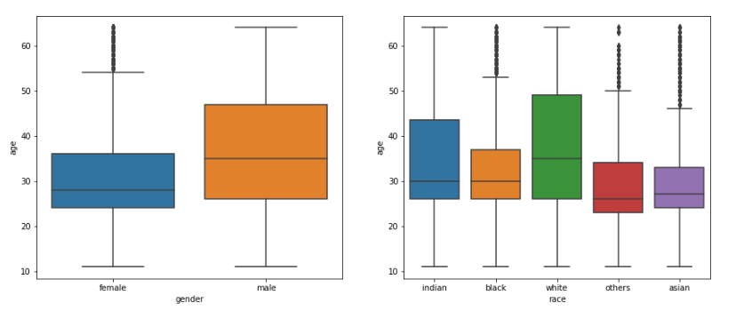
まず、次のようにして性別・人種ごとの年齢分布を調べます。
fig, (ax1, ax2) = plt.subplots(1, 2, figsize=(15, 6))
_ = sns.boxplot(data=df, x='gender', y='age', ax=ax1)
_ = sns.boxplot(data=df, x='race', y='age', ax=ax2)

すると、図のような結果になり、多くが10歳から60歳くらいであるとわかります。
年齢だけの分布を見るには
fig = plt.figure()
ax = fig.add_subplot(111)

ax.hist(df['age'], bins=50)
fig.show()
とすればよく、次のグラフが得られます。
以上の分析をもとに、10歳以上65歳以下だけ考えることにします(ちゃんと精度を上げたいなら、データの水増しの方が有効でしょう)。それが次の部分です。
# 10歳以下、65歳以上の人の画像は比較的少ないので使わないことにする
df = df[(df['age'] > 10) & (df['age'] < 65)]
次に行きます。
###### train, test, validationデータの分割
p = np.random.permutation(len(df))  # 並び替え
train_up_to = int(len(df) * TRAIN_TEST_SPLIT)
train_idx = p[:train_up_to]
test_idx = p[train_up_to:]

# split train_idx further into training and validation set
train_up_to = int(train_up_to * TRAIN_VALID_SPLIT)
train_idx, valid_idx = train_idx[:train_up_to], train_idx[train_up_to:]
この部分は実際に traintestsplit のように分割を行っているわけではなく、index を振りなおしているだけです。
###### データの前処理を行う関数
def get_data_generator(df, indices, for_training, batch_size=32):
    # 処理した画像、年齢、人種、性別をbatch_sizeずつ返す

    images, ages, races, genders = [], [], [], []
    while True:
        for i in indices:
            r = df.iloc[i]
            file, age, race, gender = r['file'], r['age'], r['race_id'], r['gender_id']
            im = Image.open(file)
            im = im.resize((IM_WIDTH, IM_HEIGHT))
            im = np.array(im) / 255.0  # 規格化
            images.append(im)
            ages.append(age / max_age)  # 最大年齢で規格化
            races.append(to_categorical(race, len(RACE_ID_MAP)))  # kerasの仕様に合わせ、one-hot表現に
            genders.append(to_categorical(gender, 2))  # kerasの仕様に合わせ、one-hot表現に
            if len(images) >= batch_size:  # メモリを考慮して少しずつ結果を返す
                yield np.array(images), [np.array(ages), np.array(races), np.array(genders)]
                images, ages, races, genders = [], [], [], []
        if not for_training:
            break
このこの部分はデータの前処理を行っています。前処理といっても大したことはしておらず、やっていることは、規格化とラベルの表現をone-hotに直すことだけです。 yield を使っているのは、メモリの上限が割と厳しいので、少しずつ渡さないとパンクしてしまうからです。
また、while True: の無限ループは学習実行時は epochs=10 のように同じ処理を繰り返す必要があるため、学習実行時のみ必要です。
続いて、いよいよモデルを構築していきます。 最終的に作りたいモデルは以下の図です。
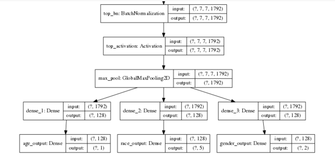
下の枝分かれしている部分(全結合層)は自分で作成し、上の畳み込み部分( EfficientNet )と結合させます。 Kerasには大きく二つの書き方があり、Sequentialモデルと、Functional API と呼ばれています。 Sequentialモデルの方は、
model = Sequential()
model.add(Dense(64, input_dim=100))
model.add(Activation('relu'))
のように、.add()メソッドを使って層を積み重ねていくようにモデルを構築できるので直感的でわかりやすい反面、柔軟性にやや劣り、複数入出力や分岐などを含む、複雑なモデルを構築するのには向いていません。
もうひとつのFunctional API は
inputs = Input(shape=(784,))
x = Dense(64, activation='relu')(inputs)
x = Dense(64, activation='relu')(x)
predictions = Dense(10, activation='softmax')(x)
のような書き方で、層一枚一枚の入出力を指定できる分、自由度の高いモデル構築が可能です。
今回作るものは、分岐が一か所入るだけの、比較的単純なものなのでどちらの書き方でも可能です。コードではFunctional APIで記述しています。
###### モデルの作成
input_layer = Input(shape=(IM_HEIGHT, IM_WIDTH, 3))  # 最初の層

efficient_net = EfficientNetB4(
    weights='noisy-student',  # imagenetでもよい
    include_top=False,  # 全結合層は自分で作成するので要らない
    input_tensor = input_layer,  # 入力
    pooling='max')

for layer in efficient_net.layers:  # 転移学習はしない
    layer.trainable = True
efficient_net の引数について説明します。 weights は初期状態でのネットワークのパラメータのことです。これはランダムでもよいですが、imagenet という画像データ群で学習させた値を使ったり、noisy-studentという学習法で学習させた値を使ったほうが、一般的に計算時間は短くなります。
include_top は畳み込み層だけでなく、全結合層もefficientnetの物を使うかどうかを決める引数です。今回は分岐という特殊な場合なので自分で作成する必要があります。
また、layer.trainable は転移学習するかどうかを決めます。した方がずっと計算時間は短くなりますが、試したところ精度が悪かったので、今回はすべてのパラメータを学習させます。
# 複数出力にする必要があるので、efficientnetの最終層から全結合層3つを枝分かれさせる
bottleneck=efficient_net.output

# 年齢の予測
_ = Dense(units=128, activation='relu')(bottleneck)
age_output = Dense(units=1, activation='sigmoid', name='age_output')(_)

# 人種の予測
_ = Dense(units=128, activation='relu')(bottleneck)
race_output = Dense(units=len(RACE_ID_MAP), activation='softmax', name='race_output')(_)

# 性別の予測
_ = Dense(units=128, activation='relu')(bottleneck)
gender_output = Dense(units=len(GENDER_ID_MAP), activation='softmax', name='gender_output')(_)

# efficientnetと全結合層を結合する
model = Model(inputs=input_layer, outputs=[age_output, race_output, gender_output])
この部分は functional API の書き方で全結合層を作成し、efficientnetと結合させています。
注意すべきは次の部分です。
# 最適化手法・損失関数・評価関数を定義してコンパイル
model.compile(optimizer='rmsprop',
              loss={'age_output': 'mse', 'race_output': 'categorical_crossentropy', 'gender_output': 'categorical_crossentropy'},
              loss_weights={'age_output': 2., 'race_output': 1.5, 'gender_output': 1.},
              metrics={'age_output': 'mae', 'race_output': 'accuracy', 'gender_output': 'accuracy'})
全結合層が3つある分、損失関数や評価関数も3つずつ定義する必要があります。 年齢の予測は回帰問題なので、平均二乗誤差、性別と人種は分類問題なので categorical cross-entropy を損失関数に使えばよいでしょう。
続く部分はバッチサイズを定義し、データを作成しています。 バッチサイズを大きくすると収束性が良くなりますが、やりすぎるとメモリがパンクするので注意しましょう。 batch_size = 64 だとうまくいかないと思います。
次です。
# 検証誤差が最も低い状態のモデルを保存しておく
callbacks = [
    ModelCheckpoint('./model_checkpoint', monitor='val_loss', verbose=1, save_best_only=True, mode='min')
]
callbacks という便利な機能を使います。これは validation data の損失関数を監視し、それが最小であったepochでのモデルを保存しておいてくれる機能です。 これにより過学習を防ぐことができます。
そして次の部分で学習を実行します。
history = model.fit_generator(train_gen,
                    steps_per_epoch=len(train_idx)//batch_size,
                    epochs=10,
                    callbacks=callbacks,
                    validation_data=valid_gen,
                    validation_steps=len(valid_idx)//valid_batch_size)
私の場合は40分ほどかかりました。気長に待ちましょう。
学習が済んだら損失関数と評価関数の値をグラフに表して学習がうまくいったかどうか確認します。
def  plot_train_history(history):
    fig, axes = plt.subplots(1, 4, figsize=(20, 5))
    axes[0].plot(history.history['race_output_accuracy'], label='Race Train accuracy')
    axes[0].plot(history.history['val_race_output_accuracy'], label='Race Val accuracy')
    axes[0].set_xlabel('Epochs')
    axes[0].legend()

    axes[1].plot(history.history['gender_output_accuracy'], label='Gender Train accuracy')
    axes[1].plot(history.history['val_gender_output_accuracy'], label='Gener Val accuracy')
    axes[1].set_xlabel('Epochs')
    axes[1].legend()

    axes[2].plot(history.history['age_output_mae'], label='Age Train MAE')
    axes[2].plot(history.history['val_age_output_mae'], label='Age Val MAE')
    axes[2].set_xlabel('Epochs')
    axes[2].legend()

    axes[3].plot(history.history['loss'], label='Training loss')
    axes[3].plot(history.history['val_loss'], label='Validation loss')
    axes[3].set_xlabel('Epochs')
    axes[3].legend()

plot_train_history(history)
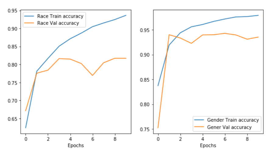
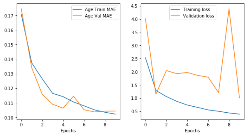
epoch 8 で何やら起こっていますが他の部分でも変動が激しいことからも確率的に起こりうることなのかもしれません。 また、特に性別と人種の分類において、かなり過学習が起こっていることが見て取れます。
最後に、各種精度に関係する値を出力し、テストデータについても予測します。
test_gen = get_data_generator(df, test_idx, for_training=False, batch_size=128)
dict(zip(model.metrics_names, model.evaluate_generator(test_gen, steps=len(test_idx)//128)))

test_gen = get_data_generator(df, test_idx, for_training=False, batch_size=128)
x_test, (age_true, race_true, gender_true)= next(test_gen)
age_pred, race_pred, gender_pred = model.predict_on_batch(x_test)

race_true, gender_true = race_true.argmax(axis=-1), gender_true.argmax(axis=-1)
race_pred, gender_pred = race_pred.argmax(axis=-1), gender_pred.argmax(axis=-1)
age_true = age_true * max_age
age_pred = age_pred * max_age

from sklearn.metrics import classification_report
print("Classification report for race")
print(classification_report(race_true, race_pred))

print("\nClassification report for gender")
print(classification_report(gender_true, gender_pred))

import math
n = 30
random_indices = np.random.permutation(n)
n_cols = 5
n_rows = math.ceil(n / n_cols)
fig, axes = plt.subplots(n_rows, n_cols, figsize=(15, 20))
for i, img_idx in enumerate(random_indices):
    ax = axes.flat[i]
    ax.imshow(x_test[img_idx])
    ax.set_title('a:{}, g:{}, r:{}'.format(int(age_pred[img_idx]), ID_GENDER_MAP[gender_pred[img_idx]], ID_RACE_MAP[race_pred[img_idx]]))
    ax.set_xlabel('a:{}, g:{}, r:{}'.format(int(age_true[img_idx]), ID_GENDER_MAP[gender_true[img_idx]], ID_RACE_MAP[race_true[img_idx]]))
    ax.set_xticks([])
    ax.set_yticks([])
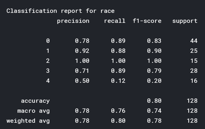
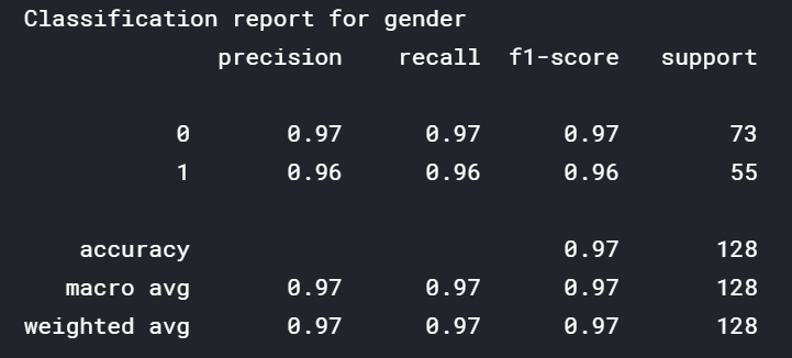
f1- score が大まかな指標になります。人種については80%の確率、性別については97%の確率で正解していることが分かります。また、学習時と比べると、過学習の傾向が強いこともうかがえます。 人種に関しては、ラベル4、すなわち 「その他の人種」についての予測が壊滅的にできていないことが分かります。
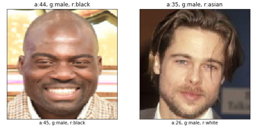
続いてテストデータのサンプルです。上が予測値、下が実際の値です。
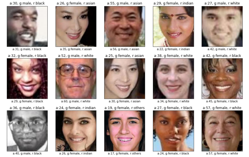
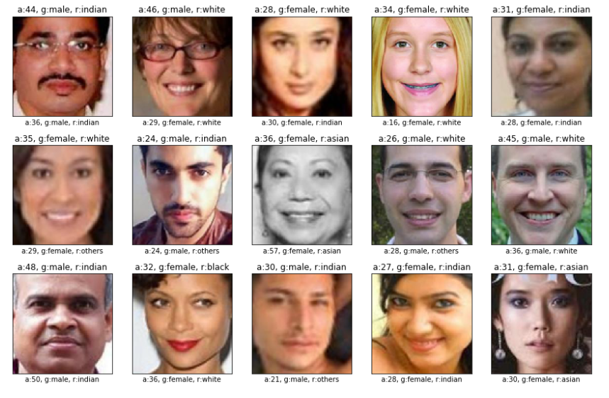
チューニングの余地がある割にはある程度予測できています。
何人か知っている人についても予測してみました。
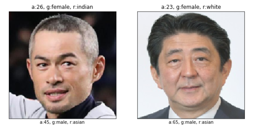
あれ.........
まとめ
今回は顔の画像から、年齢・性別・人種を同時に推定するモデルをEfficient Net を使って作りました。 今回の例のようなマルチタスク処理は、シングルタスクの精度を向上させる際にも使われることもあり、有用なので是非利用してほしいと思います。 ただ、本来EfficientNetは画像の解像度を畳み込み層の深さ・大きさと共に調節すべきものであり、今回の処理ではそれを省いているので制度は出にくい状態です。 また、画像認識の大変なところはパラメータを調節して精度を上げていくところにこそあるので、次回はこのモデルをチューニングし、過学習を抑えたりしてより精度を上げていこうと思います。
参考となるリンク先
- https://keras.io/ja/ Kerasの公式ページ、Kerasで困ったらここに来れば大体解決する
- https://sanjayasubedi.com.np/deeplearning/multioutput-keras/ モデル以外のコードを参考にした
- https://github.com/qubvel/efficientnet EfficientNet をKerasに実装してくれた人のページ、EfficientNetの内部処理はここでわかる
- https://susanqq.github.io/UTKFace/ UTKFace 公式ページ
- https://dot.asahi.com/dot/2019032200005.html イチロー引退記事、写真はここから拝借
- https://www.rbbtoday.com/article/2018/04/22/159991.html ボビーオロゴンの顔写真
- https://www.kantei.go.jp/jp/98_abe/statement/2020/0101nentou.html 安倍総理年頭挨拶。
Twitter・Facebookで定期的に情報発信しています!
Follow @acceluniverse
関連記事

概要 自分に似合う色、引き立たせてくれる色を知る手法として「パーソナルカラー診断」が最近流行しています。 パーソナルカラーとは、個人の生まれ持った素材(髪、瞳、肌など)と雰囲気が合う色のことです。人によって似合う色はそれぞれ異なります。 パーソナルカラー診断では、個人を大きく2タイプ(イエローベース、ブルーベース)、さらに4タイプ(スプリング、サマー、オータム、ウィンター)に分別し、それぞれのタイプに合った色を知ることができます。 パーソナルカラーを知るメ
はじめに この記事では物体検出に興味がある初学者向けに、最新技術をデモンストレーションを通して体感的に知ってもらうことを目的としています。今回紹介するのはAAAI19というカンファレンスにて精度と速度を高水準で叩き出した「M2Det」です。one-stage手法の中では最強モデル候補の一つとなっており、以下の図を見ても分かるようにYOLO,SSD,Refine-Net等と比較しても同程度の速度を保ちつつ、精度が上がっていることがわかります。 ※https:

はじめに まずは下の動画をご覧ください。 スパイダーマン2の主役はトビー・マグワイアですが、この動画ではトム・クルーズがスパイダーマンを演じています。 これは実際にトム・クルーズが演じているのではなく、トム・クルーズの顔画像を用いて合成したもので、機械学習の技術を用いて実現できます。 機械学習は画像に何が写っているか判別したり、株価の予測に使われていましたが、今回ご紹介するGANではdeep learningの技術を用いて「人間を騙す自然なもの」を生成する
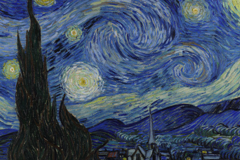
概要 DeepArtのようなアーティスティックな画像を作れるサービスをご存知でしょうか? こういったサービスではディープラーニングが使われており、コンテンツ画像とスタイル画像を元に次のような画像の画風変換を行うことができます。この記事では画風変換の基礎となるGatysらの論文「Image Style Transfer Using Convolutional Neural Networks」[1]の解説と実装を行っていきます。 引用元: Gatys et a